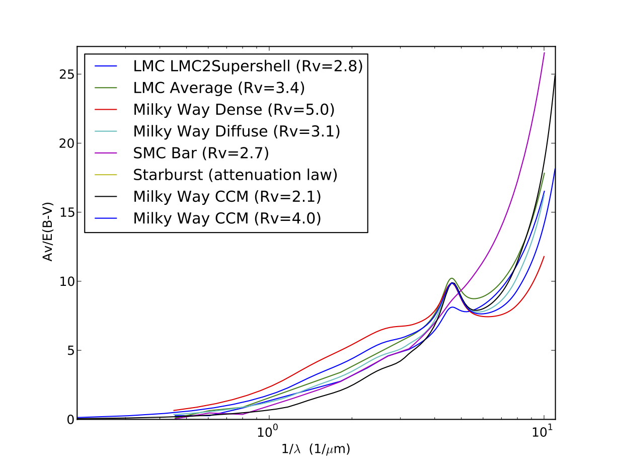
E(B-V) and the Interstellar Extinction Curves¶

The ETC supports eight different extinction relations. The Milky Way extinction curves are taken from Cardelli, Clayton, & Mathis [CCM]. In addition to curves appropriate for the diffuse and dense ISM cases, two additional curves have been added to provide more choices for Rv:

Milky Way Diffuse: An average Galactic extinction curve for diffuse ISM (Rv=3.1)
Milky Way Dense: A Galactic extinction curve for dense/molecular ISM (Rv=5.0)
Milky Way CCM1: Rv=2.1
Milky Way CCM2: Rv=4.0

The Large and Small Magellanic Cloud extinction curves are taken from [Gordon] et al:

LMC Average: Large Magellanic Cloud extinction (Rv=3.41) away from 30Dor
LMC Supershell: Large Magellanic Cloud extinction for the Supershell/in the 30Dor region but it does not apply to the 30 Dor Nebula (Rv=2.76)
SMC Bar: Small Magellanic Cloud extinction (Rv=2.74)

A general extra-galactic extinction curve is taken from [Calzetti] et al:

Starburst (attenuation law): Appropriate for stellar continuum

The following table should aid users in selecting the most appropriate extinction relation, it contains the ETC exposure times for a S/N=10 observation with a Kurucz O5 with V=15 and E(B-V)=0.4, in COS/FUV G130M/1309A through the Primary Science Aperture (PSA).

Specifically for COS, calculations for the G130M/1222, 1096, and 1055 central wavelengths should select the proper extinction laws that have wavelength coverage with these modes.

Model	Extinction	Exptime	Wavelength range
Milky Way Diffuse	Rv=3.1	308 sec	1000-22222 Angstroms
Milky Way Dense	Rv=5.0	84 sec	1000-22222 Angstroms
Milky Way CCM	Rv=2.1	612 sec	912-50000 Angstroms
Milky Way CCM	Rv=4.0	166 sec	912-50000 Angstroms
LMC Average	Rv=3.41	464 sec	998-21978 Angstroms
LMC2 Supershell	Rv=2.76	493 sec	998-21978 Angstroms
SMC Bar	Rv=2.74	3808 sec	998-21978 Angstroms
Starburst	…	92 sec	912-21997 Angstroms

Normally, the extinction factor is applied by default before the flux is normalized to the specified value in Sec.4. That is, in this case the normalized flux will correspond to the actual observed flux.

One can, however, specify an alternate computation order, in which the extinction is applied after the normalization takes place. This is useful when planning observations of targets where the “observed magnitude” is being calculated from the absolute magnitude and distance for a region of space in which there is a known, measured extinction.